This post was written (and this blog was started) with the intention of explaining a model I’ve been working on to predict future expected goals, or xG in Premier League football matches. If this sounds a bit alien, this, is an excellent primer on expected goals, and the intuition behind it all.

My reasons for doing so are multiple. My interest in this area stems from two sources, chiefly from the fact that I am a football fan, and also from a research project I undertook as an undergraduate student of statistics. My research focused on modelling future goals in football games, using a Poisson regression model, devised initially by Dimitris Karlis and Ioannis Ntzoufras [1] for Serie A football in the 1990s.

From here on gets a little technical. If you’d rather hear about the factors in my model and how I intend to use it, feel free to skip ahead.

The model’s output, essentially, was a Poisson rate parameter, for each team in each game. Much has been written on the good fit of a Poisson distribution for goal-scoring data. This parameter would then be used, with the Poisson distribution, to formulate match odds and league simulations. While the model performed relatively well, there was definite scope for improvement.

Expected goals offers far more insight into how a match actually played out. One team can be completely outplayed for ninety minutes, but get lucky and only concede one. In the last minute of injury time, they score from thirty yards. The match ends a draw. The 1-1 scoreline then goes into your data set, ready to affect the results of your analysis. This data point is definitely not representative of how the game went, and is certainly not likely to occur again. The expected goals of the match however, will give an at least slightly better picture of what actually happened and the relative strengths of the teams.

Fitted values can then act as the input to our Poisson distribution so that odds can be calculated.

The Model

One point of note is that xG data is significantly different in nature to goals scored. Obviously, goals scored must take an integer value, while xG can take any (positive) value on the real line. This makes the Poisson regression approach unworkable.

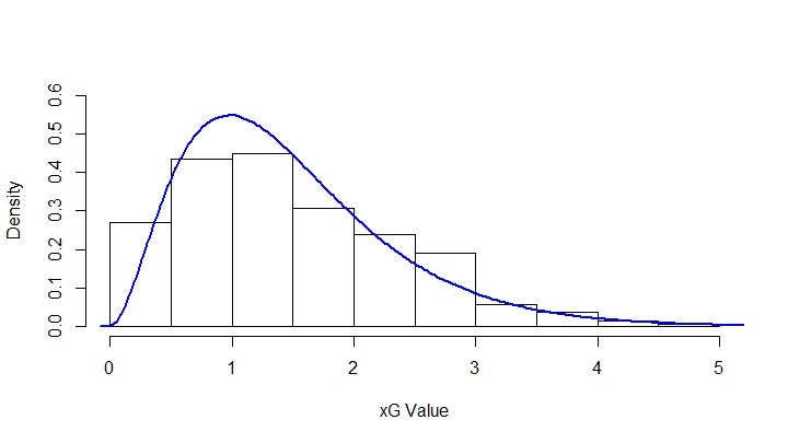
As it turns out, xG data roughly follows a Gamma distribution (below), and this ties in nicely with the fact that a Gamma prior is used in Bayesian inference for Poisson data. For this reason, a Gamma regression model was used.

More rigourously, we can use the Kolmogorov-Smirnov test to compare the cumulative distribution function of a gamma random variable to our emipirical function. The test statistic here is the largest deviation between these two CDFs and this comes to be 0.026. This correponds to a p-value of 0.31, meaning we fail to reject the hypothesis that our data is gamma distributed.

I, unfortunately, don’t have access to Opta’s, or anyone else’s feed of endless data, and so data collection was quite a painful task. WhoScored and manually collecting xG data, game-by-game, were the two means of collection.

The variables included in what I judged to be the best functioning model for the Home team’s xG in any given Premier League match were the following:

Home xG Ratio

Away xG Ratio

Home Shots On Target PG

Home xG Per Shot

Away Shots Conceded PG

Away xG Per Shot Conceded

The model for Away xG took a similar form.

The data used was the entirety of the 2016/17 season, as well as the current season to date.

Using the model, I’ll approximate the likelihood of game outcomes and the total number of goals in games, as well as forecasting forward, to predict the final league table, once a sufficient amount of the season has been played.