Cox regression is a proportional hazards model used to model ‘time to event’ data. It’s so named as a change in one of the inputs to the model results in a multiplicative effect on the hazard rate.

The haxard rate is the rate at which the event is expected to occur at time t given the event has not occured up to that point in time.

The function given by the model for the hazard rate is:

$$\lambda(t|X_i) = \lambda_0(t) exp\sum_{j}^{} \beta_j X_{ij}$$

Where $X_i$ is a vector of the $j$ covariates, $\beta_j$ is the model parameter for the covariate $j$, and $\lambda_0(t)$ is the baseline risk/hazard rate at time $t$.

The partial likelihood of the model is given by $\prod_{C_i = 1}^{} L_i(\beta)$ where the occurence of the event is denoted by $C_i = 1$

Where $L_i(\beta) = \frac{exp\sum_{j}^{} \beta_j X_{ij}}{\sum_{k: Y_k \geq Y_i}^{} exp\sum_{j}^{} \beta_j X_{kj}}$

The partial log-likelihood therefore is given by

$$\sum_{C_i = 1}^{}[(\sum_{j}^{}\beta_jX_{ij}) - log(\sum_{k:Y_k\geq Y_i}^{} exp(\sum_{j}^{}\beta_jX_{kj})]$$

And can be tidied up as:

$$\sum_{C_i = 1}^{}[\theta_i - log(\sum_{k:Y_k\geq Y_i}^{} exp(\theta_k)]$$

This expression can be maximised w.r.t to the model parameters.

Application

The dataset found here was used as an example dataset for fitting a Cox regression model.

The data relates to HR data from IBM and can be used to model employee turnover. Knowing which employees are most likely to leave, as well as the largest contributing risk factors in theory allows employers to pre-empt and/or prevent an employee leaving.

To do this the lifelines pyton package can be used. All info on it can be found here.

Note that the lifelines installation may require you to have the C++ complier for Python 2.7 found here.

# Import libraries and data
import pandas as pd
import numpy as np
import lifelines as ll
import seaborn as sns
import matplotlib.pyplot as plt

df = pd.read_csv('data/WA_Fn-UseC_-HR-Employee-Attrition.csv')

For interpretability’s sake, take a subset of the columns as features. YearsSinceLastPromotion and employee Age will be used as the predictor variables. YearsAtCompany is used as the ‘time’ variable and Attrition tells us whether they have left the company or not.

features = ['Attrition','Age','YearsSinceLastPromotion','YearsAtCompany']

# Fit the model via lifelines 
model = ll.CoxPHFitter()
model.fit(df[features], duration_col='YearsAtCompany', event_col='Attrition', show_progress=True)

model.print_summary()

    Iteration 1: norm_delta = 0.42260, step_size = 0.9500, ll = -9255.30149, newton_decrement = 215.12706, seconds_since_start = 0.0
    Iteration 2: norm_delta = 0.14466, step_size = 0.9500, ll = -9016.66007, newton_decrement = 17.72530, seconds_since_start = 0.0
    Iteration 3: norm_delta = 0.02528, step_size = 0.9500, ll = -8997.95081, newton_decrement = 0.43936, seconds_since_start = 0.0
    Iteration 4: norm_delta = 0.00190, step_size = 1.0000, ll = -8997.50740, newton_decrement = 0.00215, seconds_since_start = 0.0
    Iteration 5: norm_delta = 0.00000, step_size = 1.0000, ll = -8997.50525, newton_decrement = 0.00000, seconds_since_start = 0.0
    Convergence completed after 5 iterations.
    <lifelines.CoxPHFitter: fitted with 1470 observations, 0 censored>
          duration col = 'YearsAtCompany'
             event col = 'Attrition'
    number of subjects = 1470
      number of events = 1470
        log-likelihood = -8997.51
      time fit was run = 2019-05-07 18:08:52 UTC
    
    ---
                             coef  exp(coef)  se(coef)      z      p  -log2(p)  lower 0.95  upper 0.95
    Age                     -0.04       0.96      0.00 -10.33 <0.005     80.74       -0.04       -0.03
    YearsSinceLastPromotion -0.15       0.86      0.01 -16.12 <0.005    191.83       -0.17       -0.13
    ---
    Concordance = 0.69
    Log-likelihood ratio test = 515.59 on 2 df, -log2(p)=371.92
    

Lifelines has a model summary output method similar to that found in R, giving model summary statistics, as shown above.

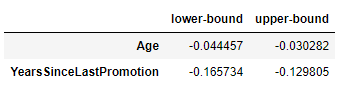
# Confidence intervals for the weight values
model.confidence_intervals_

# Interpretation of parameters
# Take age:

age_increments = range(1,50)
age_mult_effect = [np.exp(-0.04 * x) for x in age_increments]

prom_increments = range(1,50)
prom_mult_effect = [np.exp(-0.15 * x) for x in prom_increments]

sns.lineplot(x = prom_increments, y = prom_mult_effect)
sns.lineplot(x = age_increments, y = age_mult_effect)

plt.xlabel('Change in covariate')
plt.ylabel('Multiplicative effect on attrition rate')
sns.set(rc={'figure.figsize':(20,16)})
# So increases of age result in a decreased attrition rate
# Same goes for length of time since promotion.

Concordance Index

The concordance index (or C-index) is what’s commonly used to measure the goodness of fit of a survival regression model. It can be defined as the number of pairs of subjects it has correctly ordered in terms of hazard rate, relative to actual survival time. Hence, high values of C-index tell us that the model gives high-risks to subjects with a short observed survival time, and vice versa.